What Turns AI Growth Into HBM Demand?

Separating durable application demand from today’s scarcity economics.

HBM demand is booming. The memory suppliers serving it are reporting results that would have looked extraordinary at the last trough.

Reported supplier profitability snapshot — Micron.

Fiscal 2023 GAAP gross margin was −9.1%; fiscal Q3 2026 GAAP gross margin was 84.6%.
Its Cloud Memory Business Unit—covering memory solutions for large hyperscale customers and HBM for all data-center customers—reported an 83% gross margin and 78% operating margin in the quarter.

Reported supplier profitability snapshot — SK hynix.

Preliminary consolidated operating margin was 76% in Q2 2026, versus −67% in Q1 2023;
Samsung’s Memory Business said quarterly revenue and operating profit reached all-time highs.

Sources — Micron FY2023; Micron FQ3 2026; Micron CMBU scope; SK hynix Q1 2023; SK hynix Q2 2026; Samsung Q2 2026.(The scopes, periods and metrics may differ; audited HBM-only ecosystem margins are undisclosed).

The commercial moment is exceptional, but price, product mix, utilization and cost adjust on different clocks. Scarcity can lift margins before investment, yields and qualified output expand.

Added supply then erodes scarcity, and operators feel the lag across workload, qualification, budget, procurement and acceptance.

AI may have steepened demand. Supply response still operates.

The question Will this last? breaks into three parts.

Will applications keep requiring more HBM-bearing systems?
Will qualified supply remain tight?
Will supplier economics remain exceptional as capacity responds?

This article takes the first question. Article 2 takes the next two. HBM bit demand can remain structurally strong after scarcity pricing and supplier margins normalize.

1 The bridge from AI activity to HBM demand

Users, tokens, launches and gigawatt announcements signal activity.

A modelable requirement appears only when useful work is tied to its native denominator, memory signature, service target, qualified system, measured goodput, fleet policy and survivor pool.

Useful outcome → model work → native denominator + memory signature + service target → qualified system + measured goodput → fleet sizing → modeled required packages → modeled gross additions → modeled HBM attachment.

Gross additions equal required packages minus qualified survivors, floored at zero.

Qualification is the hinge: native denominator, service target and measured goodput establish what counts. The active-duty fraction stays separate; qualified survivors determine what remains to add.

FP&A — CAPITAL LENS S&OP / IBP — EXECUTION LENS

Tests timing, budget and capital alternatives. Reconciles exact configuration, inventory, supply, qualification, integration, site readiness and acceptance timing.

Together, the lenses synchronize capital timing with deployable capacity in the same planning window.

A requirement is not an order. Commitments, purchase orders, shipments, installed systems and accepted service remain separate ledgers.

Scope — This article follows AI-led demand. Argonne’s Aurora shows that simulation and data-intensive science create HBM demand.

2 Applications create different HBM-bearing work

Every application ledger follows the same scan path: PLANNING UNIT(S) → SYSTEM CONVERSION → EVIDENCE BOUNDARY. Qualification selects the attached-memory class; qualified survivors determine whether modeled additions stay positive or floor at zero.

Figure 1 shows the rule: identify the native denominator and workload stage, qualify the complete system, then follow the resulting memory path.

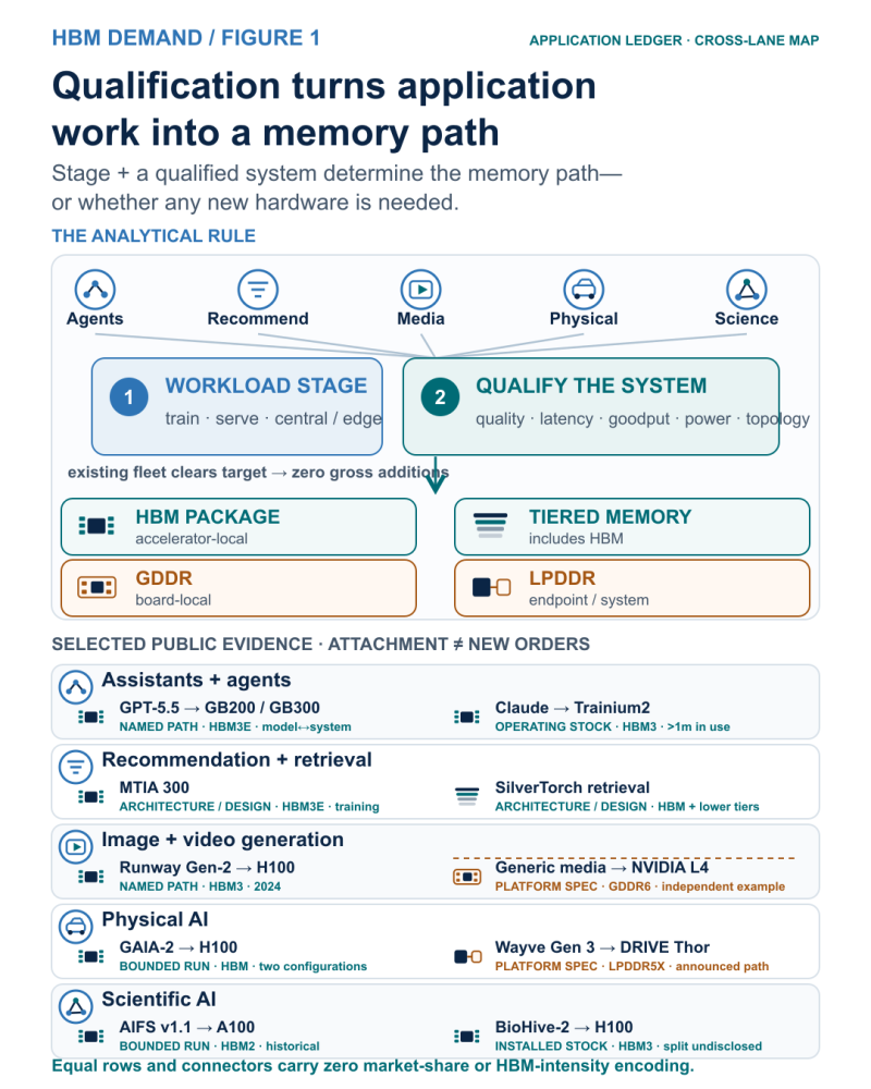
Figure 1. Each application starts with a native denominator; qualification selects its memory path. Offboard, recurring and endpoint ledgers remain separate; orders remain outside evidence.

2.1 Assistants and agents: live state sets the peak

Assistants combine resident weights, prompt processing, autoregressive decoding and retained key–value state. Agents add planning, tools, retries, revisions and independently evolving contexts. Cumulative work measures the trail; simultaneous residence measures the peak.

OpenAI names a direct model-to-system path: GPT-5.5 was co-designed for, trained with and served on NVIDIA GB200 and GB300 NVL72. GB200 joins 72 GPUs with 13.4 TB of HBM3E; GB300 provides 288 GB per GPU, about 20 TB across 72. Allocation by stage, product, region and fleet is undisclosed. OpenAI GPT-5.5; NVIDIA GB200 NVL72; NVIDIA GB300 NVL72.

Anthropic offers operating-stock evidence. In April 2026 it said it was currently using more than one million Trainium2 chips to train and serve Claude. AWS specifies 96 GiB of HBM3 and 2.9 TB/s per chip. The disclosure establishes operating stock; its split across stages, products and regions—and the purchases required to expand it—remains undisclosed. Anthropic operating disclosure; AWS Trainium2.

Anthropic reports about four times chat token use for agents and about fifteen times for multi-agent systems. These ratios measure cumulative work; concurrency and HBM attachment require separate measurement. Anthropic multi-agent system.

KV means key–value cache: attention state retained for prior tokens. In an illustration using Meta’s Llama 3.1 70B geometry—80 layers, eight KV heads, dimension 128 and two bytes each for K and V—one token contributes 320 KiB of raw logical KV. An 8,192-token context contributes 2.5 GiB; four retained together contribute 10 GiB, versus 2.5 GiB sequentially when each prior cache is released. Meta model configurations; NVIDIA inference optimization.

These totals describe raw logical state; device-HBM allocation depends on representation, distribution, placement and runtime policy. Prefix sharing and precision change representation; offload relocates blocks; eviction may trigger recomputation. Tool waits occupy HBM while state remains local; retries raise the peak when old and new state overlap. vLLM prefix caching; NVIDIA Dynamo KV offloading.

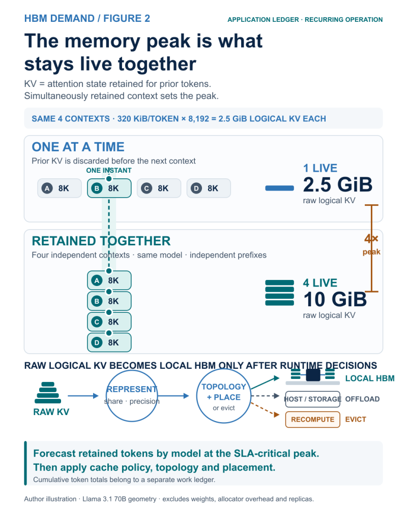
Figure 2. Four retained contexts raise illustrated raw logical KV from 2.5 to 10 GiB; physical placement and disclosed production layouts remain separate.

2.2 Recommendation and retrieval: HBM holds the hot working set

The catalogue is the warehouse. HBM is the workbench.

Recommendation combines sparse embeddings, dense parameters, jagged histories, candidate retrieval, ranking and continuously refreshed representations. Meta’s MTIA 300 carries 216 GB of HBM3E and targets training recommendation and ranking models whose embedding tables can contain more than 99% of parameters. Meta reports frequent AllReduce, AllToAll and AllGather traffic; on one 150-billion-parameter production model across 40 accelerators, its communication path was 3.9 times faster than an equivalent GPU cluster. This is direct HBM engineering evidence; installed-fleet scale remains undisclosed. Meta MTIA 300.

Meta’s GEM ads model adds scale context: several thousand current-generation GPUs and HBM pressure from embeddings, parameters and activations. After a twofold improvement, Meta reports 20–25% model-FLOP utilization. Model-FLOP utilization is the share of peak arithmetic devoted to model operations.

The remaining 75–80% covers communication, memory movement, imbalance, bubbles and recomputation. Under unchanged work, moving from 20% to 25% utilization reduces device-time by 20%; the gain can also fund larger models, faster releases or more experiments. Meta GEM.

A request narrows learned retrieval state into a shortlist while the runtime places indexes, embeddings, weights and buffers across on-chip cache, HBM, host DRAM and remote CPU-host DRAM. The shortlist is output; HBM holds selected retrieval state. SilverTorch’s A100 40 GB configuration is an evaluation case whose production-fleet scale remains undisclosed. Meta SilverTorch.

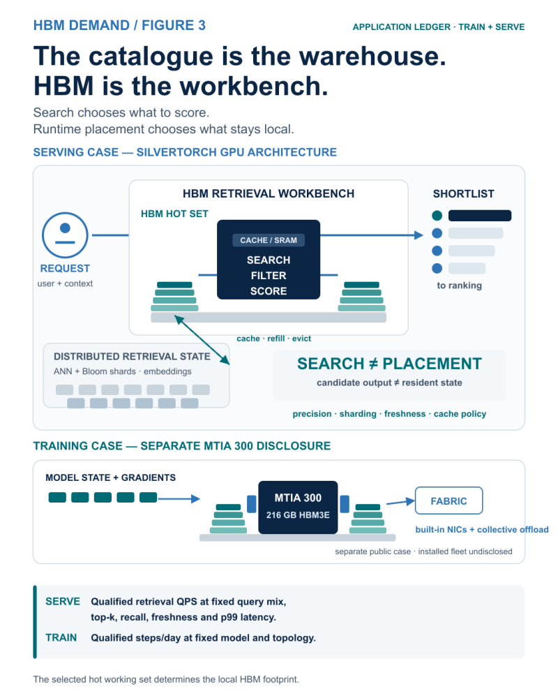
Figure 3. Search narrows candidates while placement keeps reusable state near compute; serving and training disclosures are separate, and their fleet relationship is undisclosed.

2.3 Image and video generation: work integral and residency peak

Generated media produces two hardware measures. The work integral accumulates temporal windows, sampling or refinement steps and rejected variants. The residency peak counts only state live together: weight shards, latents, activations, reusable scratch and runtime headroom. Forecast accepted images or video-minutes at fixed spatial size, duration, iteration policy, quality and deadline.

Memory reuse across disjoint lifetimes means serial work can extend accelerator-time while leaving the peak unchanged. Slicing, tiling and CPU offload exchange local capacity for time or traffic.

In 2024, Runway said A3 H100 VMs supported Gen-2 training and inference at fabric scale while GPUs per job and occupancy remained undisclosed. Separately, A3 High 8G specifies eight 80 GB H100s—640 GB aggregate nominal HBM3 across device-local memories. NVIDIA’s L4 uses 24 GB GDDR6 for video and generative workloads; accepted assets, codecs, storage and egress follow separate paths. NVIDIA TensorRT memory; Diffusers memory optimization; Runway deployment; Google Cloud GPU configurations; NVIDIA L4.

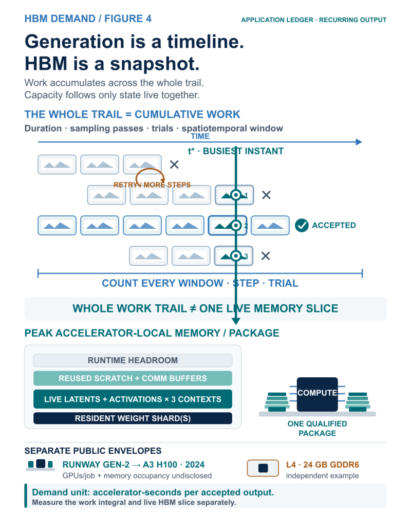
Figure 4. Generative media separates cumulative work from the live-memory peak; Runway job allocation remains undisclosed, and L4 is a separate platform example.

2.4 Physical AI: central campaigns and deployed machines

Physical AI separates offboard campaigns from onboard runtime. Wayve’s GAIA-2 report gives two training configurations: a 300,000-step, batch-128 video tokenizer on 128 H100s, and a 460,000-step, batch-256 latent world model on 256 H100s. A 20,000-step decoder GAN fine-tune omits hardware, so it remains outside the 128-H100 run.

Model the two published configurations separately; installed stock, H100 SKU, HBM per GPU, topology and elapsed hours remain undisclosed. Wayve GAIA-2; technical report; NVIDIA H100.

The endpoint evidence follows a separate lane. Wayve announced that its Gen 3 robot vehicle platform will be built on NVIDIA DRIVE AGX Thor. Public disclosures leave any GAIA-2-to-Thor model assignment undisclosed. They also leave the Gen 3 production memory bill and deployment count unresolved.

NVIDIA separately specifies one Thor SoC, 64 GB LPDDR5X and up to 273 GB/s for its DRIVE AGX Thor developer kit; treat those as developer-platform specifications rather than Wayve’s production vehicle bill.

Forecast central campaigns by accelerator-hours, completion window and overlap. Forecast endpoint attachment as qualified platforms × disclosed memory; survivors, spares and timing determine modeled additions. Wayve AV2.0; Wayve Gen 3; NVIDIA DRIVE AGX Thor.

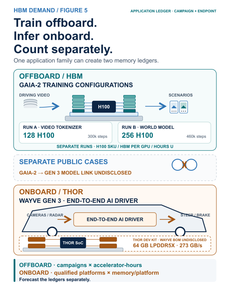
Figure 5. Physical AI creates separate offboard HBM and onboard LPDDR ledgers; model linkage, production memory and deployment count remain undisclosed.

2.5 Scientific AI: three demand clocks

Scientific AI runs on three clocks across owned, rented or shared fleets: training campaigns by qualified work and deadline; operational forecasts by on-time issuance plus reserve; and discovery loops by accepted experiments per lab-compute cycle. Each clock counts different work; combine mapped, compatible schedules.

ECMWF’s AIFS Single v1.1 model card discloses 64 A100 GPUs with 40 GB each for about one week. Converting one week to seven days gives roughly 448 A100-device-days by author arithmetic. That figure covers the disclosed training procedure; full program work and annual cadence remain outside its scope. ECMWF AIFS Single v1.1.

AIFS Single v2 entered operations on 12 May 2026. It issues one 15-day global trajectory with 6-hourly outputs four times daily. Training used 16 120 GB GH200 GPUs for about four days; the production fleet, allocation, reserve and purchases remain undisclosed.

AIFS ENS v2 is separate: 51 members trained on 32 GH200 GPUs for about one week. Keep the denominators separate. ECMWF AIFS Single v2; ECMWF AIFS ENS v2; ECMWF operational dataset status.

Recursion discloses BioHive-2 as installed infrastructure: 63 DGX H100 systems, 504 H100 GPUs and Quantum-2 InfiniBand. NVIDIA specifies eight 80 GB H100 GPUs, or 640 GB aggregate HBM3, per DGX H100; 63 systems therefore imply 40.32 decimal TB of nominal aggregate HBM3. This is distributed installed stock; pool capacity, consumption, allocation and scientific throughput require separate evidence.

“Accepted experiments per lab-compute cycle” is author-defined; BioHive-2 discloses installed infrastructure. Keep device-days, operational issuances and lab outcomes separate.

Map each lane to qualified replicas by configuration, deadline and time bucket. FP&A can then compare owned, rented or reserved capacity across compatible schedules. Recursion BioHive-2; NVIDIA DGX H100.

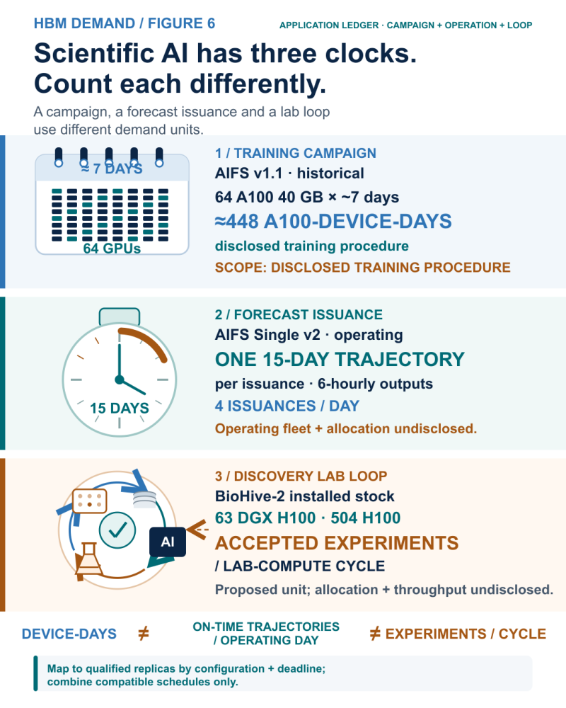
Figure 6. Scientific AI uses separate training, forecast and lab denominators. Map by qualified configuration and deadline; operating allocation and lab throughput remain undisclosed.

3 Four memory-system jobs determine qualified goodput

HBM is one component inside a qualified path. Four modular jobs determine qualified goodput: HOLD capacity, FEED compute, EXCHANGE distributed state and TIER colder state. Every required job must clear the same operating boundary.

Figure 7 separates two planning questions on the same qualified configuration. RUNTIME QUALIFICATION measures accepted work per active replica within quality, latency, availability, software, topology, power and thermal limits. DEPLOYABLE SUPPLY asks how many compatible complete systems can be manufactured, allocated, integrated, sited and accepted by date; HBM and logic availability, packaging yield, substrates and test bind that ledger. TSMC CoWoS; AMD CDNA 3.

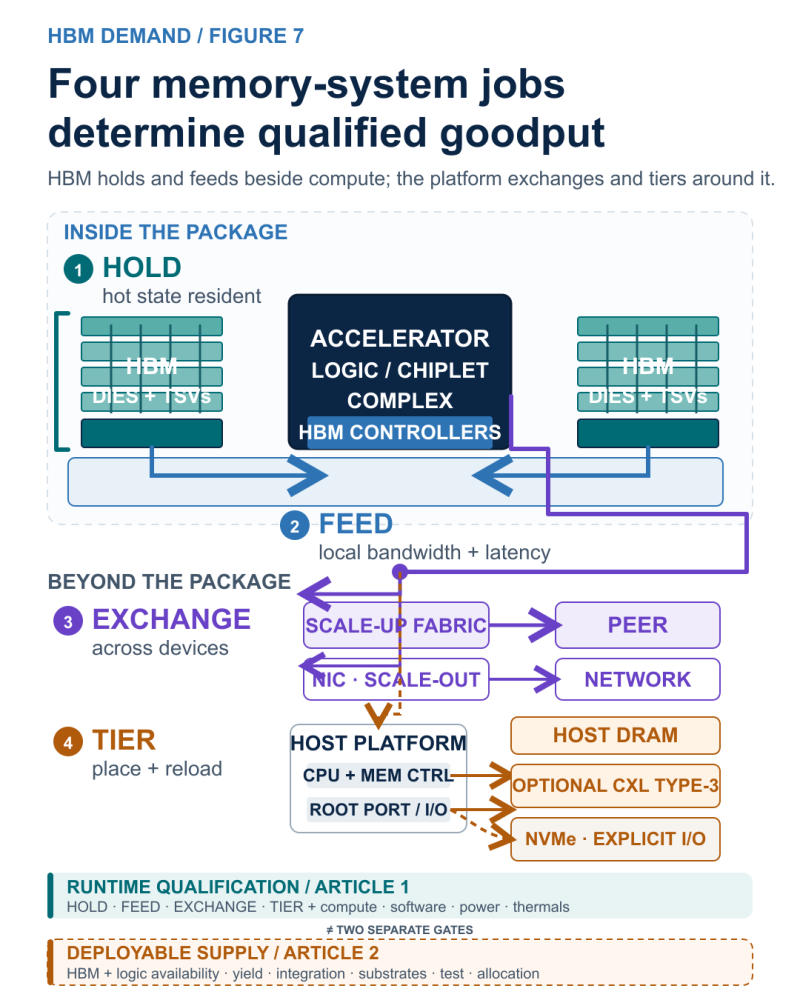
Figure 7. Runtime qualification measures accepted work; deployable supply counts compatible systems manufactured, allocated, integrated, sited and accepted by date.

HOLD — Capacity. Peak simultaneous state sets capacity; lifetime bytes belong to the work ledger. Agents retain weights, live KV and runtime buffers. Recommendation keeps the latency-critical hot set. Media holds live tensors and workspaces. Central physical-AI and scientific runs retain model, batch or simulation state. Other catalogues, completed assets, archives, datasets and endpoint windows usually occupy larger tiers.

FEED — Delivery. Fit establishes capacity; sustained byte delivery establishes feed. Decode rereads weights and KV; recommendation gathers and refreshes sparse state; media updates spatial and temporal tensors; training and science move activations, gradients, optimizer state, fields and buffers. The sustained access pattern determines whether the target clears. Roofline treatment.

EXCHANGE — Topology. Scale-up coordinates shards and collectives; scale-out connects nodes and replicas. Disaggregated serving can turn KV into a network payload. A constrained fabric can strand installed HBM or reduce useful output. Splitwise; NVIDIA Dynamo.

TIER — Placement. HBM serves hot state; SRAM, host DRAM, optional CXL Type-3 memory and NVMe or remote storage serve other patterns. Runtime policy promotes, evicts, prefetches, pins, recomputes or offloads. NVMe uses explicit I/O; DRAM and CXL use load/store semantics. Tiering saves HBM only when reload or recompute meets the target. NVIDIA GPUDirect Storage; CXL 3.0 specification.

Key distinction — qualified goodput is the result. It measures useful work per active replica on the full configuration at the required quality, latency or deadline and placement. Failover remains a qualification test. The planned active-duty fraction separately states the installed share expected to serve simultaneously; apply it once. More HBM leaves output unchanged when fabric, reloads, compute, software, power or thermals bind first.

3.1 Fit is necessary; qualified goodput decides

In an illustrative two-package 70-billion-parameter replica, evenly shard two-byte weights and logical KV. Each package holds 70 decimal GB of weights plus approximately 48.318 decimal GB of KV for 64 live 4,608-token sequences. Add a hypothetical 20 decimal GB runtime allowance: 138.318 decimal GB per package.

A 200 decimal GB package with 10% reserve provides a 180 decimal GB budget and 41.682 decimal GB headroom. This establishes fit; full-system qualification supplies fleet-bridge performance and eligibility. Meta model configurations; vLLM memory categories.

Sharding sets packages per replica; replication sets replica count—forecast topology, then packages and HBM.

4 The fleet bridge: from qualified work to a modeled requirement

Here engineering hands qualified goodput to planning. The bridge produces a modeled hardware requirement; FP&A and S&OP/IBP synchronize capital timing and deployable capacity against one deployment window. An order still requires operator action.

Active replicas: round up workload ÷ qualified goodput.
Installed replicas: divide by planned active-duty fraction and round up.
Required packages: multiply by packages per replica.
Modeled gross additions: subtract complete qualified survivors once and floor at zero. Multiply by HBM per package for modeled new attachment.

Consider a hypothetical recurring scientific-forecasting service—not an ECMWF fleet disclosure. Its workload unit is one forecast-member trajectory delivered by the deadline.

Workload. One deadline window requires 960 on-time forecast-member trajectories.
Active fleet. Assume a two-package replica with 200 GB of HBM per package. At qualified goodput of 2.0 on-time trajectories per deadline window per active replica, the service needs 480 active replicas.
Installed fleet. A planned active-duty fraction of 80% requires 600 installed replicas, or 1,200 packages.
Survivors. Start with 1,000 opening packages. Retirement, reassignment or incompatibility removes 100 from this application lane, leaving 900 qualified survivors that form 450 complete, assignable two-package replicas in the same lane.

Amazon reports accounting lives of five to six years for servers and networking equipment; Meta reports five to 5.5 years. Those schedules differ from operational eligibility, which follows memory fit, topology, software support, power and SLA. Amazon 2025 Form 10-K; Meta 2025 Form 10-K.

Modeled addition. The baseline requires 300 gross package additions, or 60 decimal TB of new HBM attachment. FP&A compares deployment date, budget and owned-versus-rented options. S&OP tests whether exact packages can be sourced, qualified, integrated and accepted in time. Orders, shipments and installed stock remain separate ledgers.

Now vary qualified goodput alone.

Higher-goodput case. At 2.5 on-time trajectories per window per active two-package replica, the fleet needs 960 packages and 60 gross additions containing 12 decimal TB.

Lower-goodput case. At an illustrative 1.6 on the same denominator, the fleet needs 1,500 packages and 600 gross additions containing 120 decimal TB.

Hold workload, topology, active-duty fraction, HBM per package and 900 qualified survivors fixed. A 20% goodput decline, 2.0→1.6, raises required packages 25%, 1,200→1,500. The same survivor subtraction doubles the gap: max(0, 1,200−900)=300; max(0, 1,500−900)=600.

Key distinction — in this one-factor case, a 20% goodput decline raises required packages 25% and modeled gross additions 100% against 900 qualified survivors.

The doubling is specific to this survivor ratio. Figure 8 shows the full bridge and its fixed-fleet sensitivity.

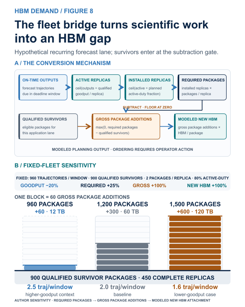
Figure 8. Only goodput varies; with 900 qualified survivors, a 20% drop raises required packages 25% and modeled gross additions 100%. Doubling is ratio-specific; ordering requires action.

5 Each optimization changes a different system ledger

Exact-prefix reuse changes repeated model work and, where the runtime physically shares blocks, duplicate local KV residence. Tiering changes placement and transfer traffic. Software and scheduling change accepted work per active replica. Replatforming changes the complete compute–memory system.

Each lever creates a changed integrated configuration whose HBM effect appears only after requalification on the same model, precision, workload mix, quality, tail-latency target, availability and topology.

Prefix caching spends cache capacity to skip repeated prefill while decode continues. In the fixed attention example, sixteen 4,608-token sequences containing the same exact 4,096-token prefix occupy 22.5 GiB with independent copies. Perfect physical block sharing reduces the arithmetic total to 3.75 GiB—an upper bound of 18.75 GiB. Measured savings depend on prefix overlap, hit distribution, eviction, transfer bandwidth and the SLA. vLLM prefix caching.

KV offload relocates reusable blocks from HBM to host memory or storage and later reloads them. Lower local residence is exchanged for transfer traffic, lower-tier capacity and latency. Host DRAM and optional CXL-attached memory are memory tiers; SSD is storage. NVIDIA Dynamo cache offload; CXL active memory tiering.

Platform crossover thresholds are workload-, SLA- and system-specific. NVIDIA’s H200 offers an HBM3e envelope; its RTX PRO 6000 Blackwell Server Edition uses GDDR7 for enterprise AI, graphics and simulation; Jetson Thor uses LPDDR5X at the edge. These are complete architecture envelopes with tightly coupled compute, memory, software, power and topology choices. Replatforming can also change packages per replica and which opening systems remain qualified survivors. H200; RTX PRO 6000; Jetson Thor.

Custom silicon can continue using HBM: Trainium, Google TPUs and Microsoft Maia provide examples. Complete architecture determines the memory path. Google TPU v5p; Maia 200.

At fixed approved work, requalify and recompute the fleet gap: the first-order effect. A passing change can lower residence, reduce or defer packages, or redirect work. Figure 8’s ceilings, complete-replica survivors and zero floor still govern; failure leaves the baseline requirement.

Lower cost creates an option, not automatic demand. Rebound enters only after an operator approves additional work as a separate second-order scenario and reruns the bridge.

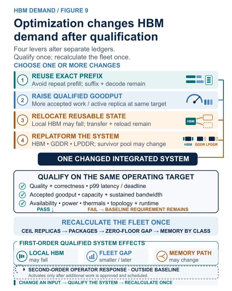
Figure 9. Qualified system changes drive first-order fleet effects; rebound requires operator-approved work, and package reduction requires measured fleet impact.

The watchlist

1. Workload and memory signature: accepted outcomes, model executions and simultaneous resident state.

2. Qualified service performance: quality, percentile latency or deadline and goodput on the actual topology.

3. Fleet conversion: active and installed replicas, modeled required packages, qualified survivors, modeled gross package additions and modeled new memory attachment by class.

4. Commercial conversion: approval, commitment, purchase order, shipment, installed system and accepted service, each with its date and quantity.

Article 1 ends at a modeled gross hardware requirement: packages by named configuration, location and deployment date. The requirement becomes a commercial order only when an operator issues a purchase order or draws against an approved commitment.

Article 2 asks how many exact systems can clear the memory, logic, stack, package, test, platform and site gates in the same period—and what happens to supplier economics as capacity responds.

Which gate do you expect to bind next: memory, advanced packaging, platform qualification or site power?